
|
Draft for Information Only
Content Kinematics: Tangential Motion in Space
Kinematics: Tangential Motion in SpaceLike motions in 2D practical engineering problems, sometimes it is convenient to resolve the component functions of the vector function of a 3D motion into components which are tangent and normal to the path of the motion. Thus the study of the motion can be focused on the tangential motion of an object as the velocity vector of the motion of an object is always tangent to the path of the motion of the object. This is only a method to study the motion of a particle along the path not a rigid coordinate system to specify the position of the particle. Tangential and Normal Component FunctionsIn curvilinear motion, when the vector function of motion is resolved into component functions that are tangent and normal to the path of motion, the orientation of the frame of reference of the object changes during the motion along the path. In other words, the reference frame of the object is in translative and rotational motions simultaneously along the path of motion. However, there are an infinite number of normal component function prependicular to the tangent component at a given point of the tangential motion in space. Similar to curvilinear motion in 2D, an osculating plane is defined at the given point by constructing a plane parallel to the plane defined by the unit tangential vector at the given point and the differential change of the unit tangential vector at the given point with its neighborhood unit tangential vector. 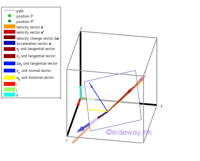
Since the velocity vector of the motion is alway tangent to the path, the vector function of the velocity vector does not have both normal and binormal velocity components. However the vector function of the acceleration vector have both tangential and normal acceleration components such that the speed of the tangential velocity vector can be accelerated by the tangent component of the acceleration vector and the direction of the tangential velocity vector can be accelerated by the normal component of the acceleration vector. In general, by taking the limit, the component of the acceleration vector along the binomal is equal to zero. By definition, the osculating plane at a given point is always parallel to its neighborhood unit tangential vector. When taking limit, the osculting plane at a given point will fit closely to its neighborhood unit tangential vector and it neighborhood point will also move much closely to the given point. Therefore the motion at the osculating plane obtained in the limit can be considered as a 2D motion with the binomal acceleration component equal to zero. Let et be the unit tangential vector at the osculating plane. There always exists a unit normal vector en at the osculating plane also. Further, as the limit of the vector Δet/Δθ is equal to en, the unit tangential vector at the osculating plane is called principal normal at a given point. Once the directions of unit tangential vector et and principal normal vector en are defined, the unit principal binormal vector eb which is equal to the cross product unit tangential vector and principal normal vector, can also be defined to form a right-hand triad accordingly. And the binormal vector is therefore perpendicular to the osculating plane also in the limit. 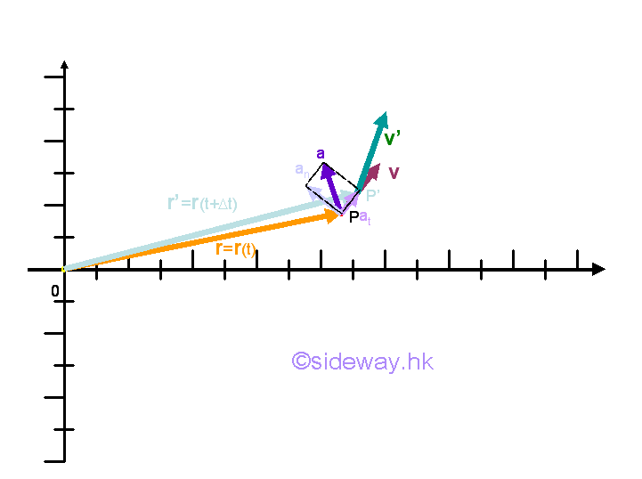
Let the unit vector tangent to the velocity vector v be et and the unit vector normal to the velocity vector v be en. Unlike the unit vectors i and j of the fixed frame of reference, the unit vectors et and en are translated and rotated simultaneously along the path of the motion. Assuming the motion of an object at position P at an instant of time t undergoes a motion of velocity v with an angle of θ relative to the x-axis of the fixed frame of reference. After time interval Δt, the object moves along the path with path length equals to Δs to position P' at which the object undergoes a motion of velocity v' with an angle of θ+Δθ relative to the x-axis of the fixed frame of reference at the instant of time t+Δt. Therefore both the magnitude and direction of the velocity vector is a function of angle c and in turn a function of time t. As the time interval Δt approaching zero, the path length Δs can be approximated by ρΔθ where ρ is the radius of curvature at position P and is appoximately equal to the radius of curvature at position P'. 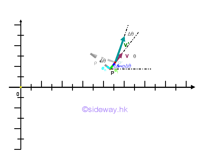
Therefore the velocity vector v at position P can be expressed in term of the tangential and normal unit vectors, that is v=0en+ vet where v is the scalar function of the velocity vector v tangent to the path and magnitude 0 is the scalar constant of the velocity vector v normal to the path at position P. As the velocity vector v does not have normal component, velocity vector v is equal to the product of the scalar function v and the unit vector et only, that is v=vet. The acceleration of the object at position P can be obtained by differentiating the velocity vector function with respect ot time t. Imply 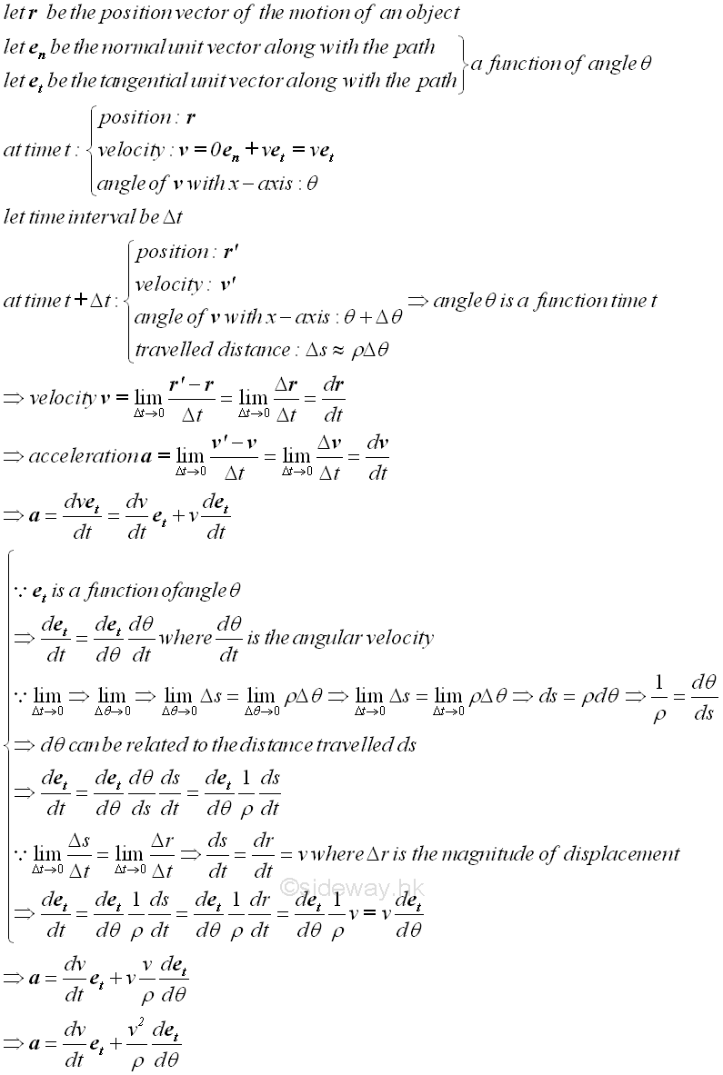
The acceleration vector a at position P can be decomposed into a tangential component function and a component function of the rate of change of the tangential unit vector et with respect to the angle c. In fact the rate of change of the tangential unit vector et with respect to the angle c when taking limit as Gc approaching zero is equal to the vector normal to the tangential unit vector et which implies that the acceleration vector a at position P can be resolved into a tangential component function and a normal component function. Graphically, the rate of change of a tangential unit vector et is 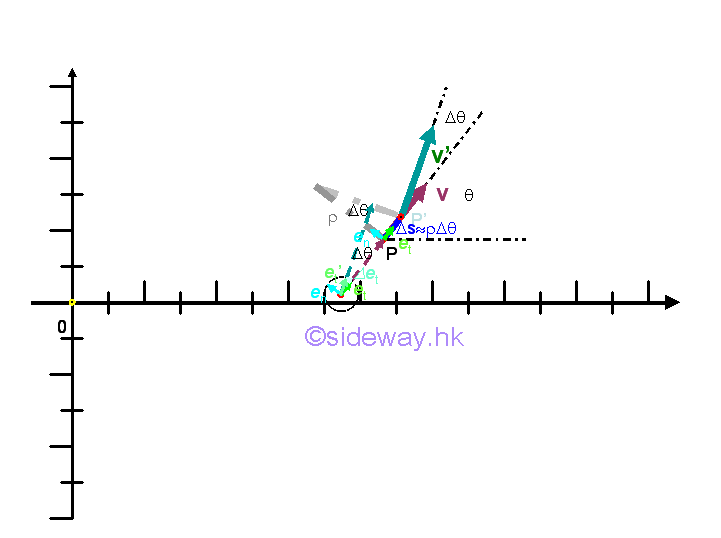
Since the rate of change of a tangential unit vector et when taking limit as Gc approaching zero is only due to a vector normal to the tangential unit vector et, with magnitude of the normal vector equals to 1, that is the rate of change of the tangential unit vector et with respect to the angle c when taking limit as Gc approaching zero is equal to the normal unit vector en. Imply 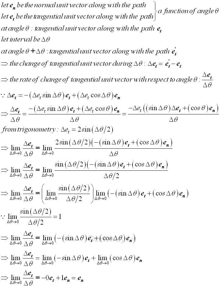
Therefore the acceleration vector a at position P can be resolved into a tangential component function and a normal component function. Imply 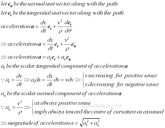
©sideway ID: 140900001 Last Updated: 9/7/2014 Revision: 0 Ref: References
Latest Updated Links
  Nu Html Checker Nu Html Checker  na na |
 Home 5 Business Management HBR 3 Information Recreation Hobbies 9 Culture Chinese 1097 English 339 Travel 45 Reference 79 Hardware 55 Computer Hardware 261 Software Application 213 Digitization 37 Latex 52 Manim 205 KB 1 Numeric 19 Programming Web 289 Unicode 504 HTML 66 CSS 65 SVG 46 ASP.NET 270 OS 431 DeskTop 7 Python 72 Knowledge Mathematics Formulas 8 Set 1 Logic 1 Algebra 84 Number Theory 206 Trigonometry 31 Geometry 34 Calculus 67 Engineering Tables 8 Mechanical Rigid Bodies Statics 92 Dynamics 37 Fluid 5 Control Acoustics 19 Natural Sciences Matter 1 Electric 27 Biology 1 |
Copyright © 2000-2026 Sideway . All rights reserved Disclaimers last modified on 06 September 2019