
|
Draft for Information Only
Content
Functions and Models
Functions and ModelsIn general, a function f can be defined as the relationship between two variables, i.e. the input variable and the defined one-to-one permissible output variable. A model or mathematical model is the using of function, mathematical equation, to represent a physical problem. Constants and VariablesConstants are usually used as the term for numbers in the algebraic expression to represent the one with a fixed amount of quantity. But sometimes symbols, for example, letters, in the algebraic expression are also used to disguise a fixed amount of quantity instead of using the actural number. Therefore, symbol in an algebraic equation can also be a kind of constant when the symbol is used to represent a fixed amount of quantity in an algebraic expression. Unlike a constant number, a symbol can represent one or more numbers in the algebraic expression. However the representing quantity of a symbol in the algebraic are only varied with the applicaion of interest. For example, the motion equation for the case of constant acceleration can be applied to any constant acceleration motions 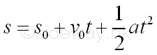
The motion equation of constant acceleration can be applied to any constant acceleration motions by substituting the corresponding initial displacement sment s0, initial velocity v0, and uniform acceleration a into the equation accordingly. The displacement s and time t in the algebraic expression are not constants but variables because the values of these variables can be more than one number. For example, the time t can begin from 0 and then increases to any value, while the distance s will be varied accordingly. Limitation/Range of VariableIn general, the range of a variable in an algebraic equation for a physical problem are limited. For example, the Ideal Gas Law, PV = nRT where P is pressure of the gas, V is volume of the gas, n is the amount of the gas in term of number of moles, R is the ideal or universal gas constant, and T is the absolute temperature of the gas. When pressure P remains unchange and the temperature T is lowered to absolute zero, the volume V must be zero also. This is not true, because this is only true for an ideal gas. For real gas, the properties of a real gas begin to deviate from the ideal gas law at low absolute temperatures close to absolute zero. Thermal energy is involved in the condensation of gas under pressure and all real gases liquify above absolute zero. Liquid does not obey the ideal gas law and therefore all real gases disobey the ideal gas law at low absolute temperature. The values of the variable temperature T cannot be lowered to the level of low absolute temperatures close to absolute zero also. Usually, the limitation or range of a variable can be expressed as.
a and b can be any number, if there is no limitation on x, then the range of x can be expressed as -∞<x<∞. Since variable x can be any number between a range, the variable x is called continuous variable. There is also variable that is not continuous and is called discrete variable. For example, sum of a geometric serie, Sn=a+ar+ar2+...+arn-1, the variable n can only be positive integer and is called integer variable. Functions & VariablesThe algebraic expression of the constant acceleration motions is the relation between the variable s and t. When the variable time t in the algebraic expression is increased, the variable distance s in the algebraic expression is increased also. The variable time t in the algebraic expression is called independence variable because the value of time t can vary freely between the range. The variable distance s in the algebraic expression is called dependence variable because the value of distance s is the output effect depending on the variable time t. In other words, variable distance s is a function of the variable time t, or expressed as s=f(t) symbolically to represent that s is a function of t. The relation between the two variable should refer to the algebraic expression itself so that the value of s can be determined from the value of t. The limitation of the independence variable in a function is called the domain of function. While the functional values of the dependence variable of a function is called the range of function. Since a function is defined as a relation between two variable only, when variable s if a function of variable t, variable t is also a function of variable s. For the algebraic expression of a constant acceleration motion, the distance s is determined by time t, and is so called distance s is a function of time t, e.g. s=f(t). If this relation is defined as the normal function between the two variable, then the algebraic expression of the relation between s and t in term of s, that is the time t is determined by distance s and is so called time t is a function of distance t, e.g. t=f-1(s), the inverse function of the two variable. some typical examples of normal functions y=x2, y=sin x and y=log x and the corresponding inverse functions x=√y,x=sin-1y and x=10y. When the algebraic expression of the relation between two variables can be formulated by expressing the dependent variable in terms of the independent variable explicitly is called explicit function. The algebraic expression of a constant acceleration motion is an explicit function. However, sometime the algebraic expression of the relation between two variables cannot be formulated by isolating the dependent variable from the independent variable on one side of the algebraic expression. When both the dependent variable and independent variable are mixed on one side of the equation, for example, x2 + xy + y2 = 0, the function is called implicit function. A function in more general sense only defines the relation between two variables, there is no more information about the two variables themselves. Although a single-valued or monodromy function has an unique value of dependence variable in the range for each value of independence variable within the limitation. Sometimes the dependence variable may not have a solution for an independence variable outside the limitation. For example, y=log x, y is a function of x, but when x<0, there is no solution. Besides, a function called multiple-valued function can have more than one functional value of dependence variable corresponding to each value of independence variable. For example, y2=x, y is a function of x, therefore the dependence variable y can be expressed as two single-valued function y=√x and y=-x. Types of FunctionsFunctions can be classified into different catalogs according to their characteristic and properties. Besides, the normal function and inverse function, the implicit function and explicit function, the single-valued function and the multiple-valued function, some other common classifications of functions are:
As a function is used to describe a relation between two variables, sometimes, a function cannot be expressed in terms of one simple mathematical equation. A function is called elementary function when a function can be constructed by using a finite combination of the basic building blocks, the simplest elementary functions and elementary operations. Both algebraic function and transcendental function are elementary functions. However, not all functions are elementary function. For example, a piecewise-defined function usually uses more than one equations to define the relation between the dependent variable and independent variable. A function is called non-elementary function or special function when a function is not an elementary function. The types of elementary functions can be classified as following:
Number and Number Line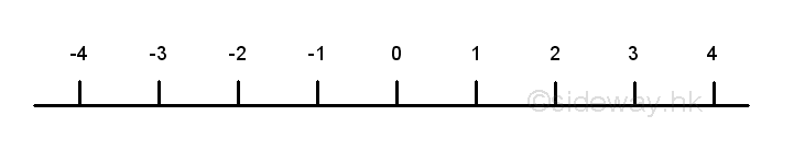
The vaule of a independent variable can be graphically represented on a number line. After defining a position on the straight line as the zero point and a unit length of the straight line as one unit length, then points can be added starting from the zero point on the line through marking the unit length on the line repeatedly. Each point is associated with the number of counting the unit length with positive numbers are to the right of zero and negative numbers are to the left of zero. Numbers are orderly located on the line geometrically with the number on the right is always greater than the number on the left. Number to the right of zero is the counting numbers e.g. 1,2,3... and is called natural numbers. Sometimes zero is included to the set of natural numbers N, but the set of number including zero is called Whole number. And the set of numbers marked on the number line of one unit length apart starting from zero, e.g. -3,-2,-1,0,1,2,3, is called integer Z. An integer is also called a whole number, which can be positive, negative, or zero. Numbers can then be grouped into
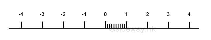
Since the unit length between two successive numbers is not equal to zero, more numbers can be inserted between points of integers. The most effective method of inserting point to the line segment is by method of equal division. For example, 9 more points or numbers can be obtained by dividing the number between 0 and 1 into ten equal divisions, the numbers from left to right are 0.1=1/10, 0.2=2/10,...,0.9=9/10. More numbers on the number line can also be obtained similarly, e.g. 1/3, 2/3. The numbers on both end can be expressed as a fraction p/q, e.g. 0=0/10, 1=10/10. These numbers are called rational numbers Q, which can be expressed as a fraction p/q where p and q are integers, q0, and p and q have no common divisor other than one. 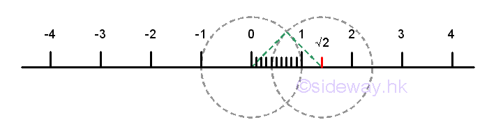
Although, much more points can be plotted on the number line using the method of equal division, the rational number points cannot fill up the number line. There are points on the number line that cannot be expressed as a fraction p/q. For example, √2. The position of the point √2 on the number line can be located using the pythagorean theorem by constructing a right angle triangle with two sides equal to one unit length with the hypotenuse equals to √2. The point at √2 is not a rational point and can be proved by contradiction. If √2 is a rational , then √2 can be expressed as a fraction p/q. Imply 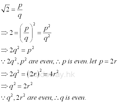
Both p and q are even, 2 is a common factor of p and q. Through the repetition of steps, 2 is always the common factor of the numbers generated. Since p and q always have an even common factor, this contradicts the definition of rational and the assumption that √2 is a rational is false. The point cannot be expressed as a fraction p/q is called irrational point. There are many other examples of irrational points, for example, √3, √5,... Numbers associated with these irrational points that cannot be expressed as a fraction p/q numbers are called irrational number I. Therefore √2 is an irrational number. There are many other types of irrational numbers, for example, π, e,... The set of rational numbers Q and the set of irrational numbers I together form the set of real numbers R. Continuous Variables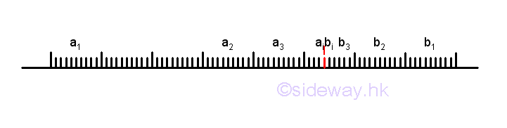
A continuous variable is the one for which any value, even infinitive small segmented value, is possible within a given limitation. In other words, there are infinitely many possible values for a continuous variable within a given limitation. Geometrically, the point of a continuous variable can vary along the number line passing through all rational points and irrational points continuously without any jumping. For example, the value of a continuous variable with limits 1≤x≤2 can be any number between 1 and 2. The value of a rational number can be determined by the fraction of the corresponding numerator and denominator. The irrational number √2 can be one of the possible value. Although the value of an irrational point cannot be determined by a fraction directly, the value of an irrational point still can be estimated by the position of the irrational point on the number line relative to the nearby rational numbers. Since both rational points and irrational points lie on the same line, two rational point a1 and b1 on the number line can be selected to bound the interested irrational point I. Although the irrational point is confirmed to be located within the line segment a1b1, the actual position is not known because there are many other rational points and irrational points on the line segment. In order to increase the accuracy, the length of the line segment can be reduced by selecting another two rational points a2 and b2 inside the line segment a1b1 to bound the irrational point I. Since the irrational point I is located within line segment a2b2 and line segment a2b2 is shorter and is included line segment a1b1, the estimation of the position of irrational point I on the line segment would be more accurate because those irrational points lies on line segment a1b1 and outside line segment a2b2 will be elimated. Repeating this elimination process by selecting another set of rational points ai and bi to reduce the length of the line segment aibi, the position of the irrational point I would become much more accurate. By repeating the elimination process infinitely, the line segment anbn can be reduced to approaching zero, and the position of the irrational point I on this infinitely small point can then be defined by the estimation process using two group of rational point on the number line, i.e. lower limit a1, a2, ..., ai, ..., an and upper limit b1, b2, ..., bi, ..., bn. Therefore the value of the irrational number associated with the irrational point 2 can also be estimated similarly. 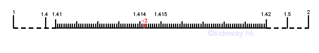
Since the square of 1 is smaller than 2 and the square of 2 is greater than 2, imply the value of irrational number √2 must be between 1 and 2. Select another set of rational numbet to reduce the length of the number line segment. The square of 1.4 is smaller than 2 and the square of 1.5 is greater than 2, imply the value of irrational number √2 must be between 1.4 and 1.5. Similarly, the value of irrational number √2 must be between 1.41 and 1.42, and between 1.414 and 1.415, and between 1.4142 and 1.4143, and ....etc. Therefore the value of irrational number √2 can be estimated by two groups of rational numbers, i.e. lower limit 1,1.4,1.41,1.414,1.4142,... and upper limit 2,1.5,1.42,1.415,1.4143,... Since the difference of the two selected groups of rational numbers is the last digit of the upper limit is always greater than the lower limit by one in order to bound the irrational number, the upper limit can be ignored as the upper limit is pre-defined. The value of irrational number √2 can be estimated by the group of the low limit rational numbers. The group of the low limit rational numbers can be expressed as a generalized representation, i.e. 1.4142... and the value of irrational number √2 can also be expressed as an unique infinite decimal expansion and written as 1.4142.... However not all numbers with unique infinite decimal expansions are irrational number because all rational numbers have either finite decimal expansions, e.g. 1/2=0.5 or infinite repeating decimal expansions, e.g. 1/3=0.3333...=0.3. Only those numbers with infinite decimal expansions with endless non-periodic decimal dights to the right of the decimal point. Graphical Represent of a Function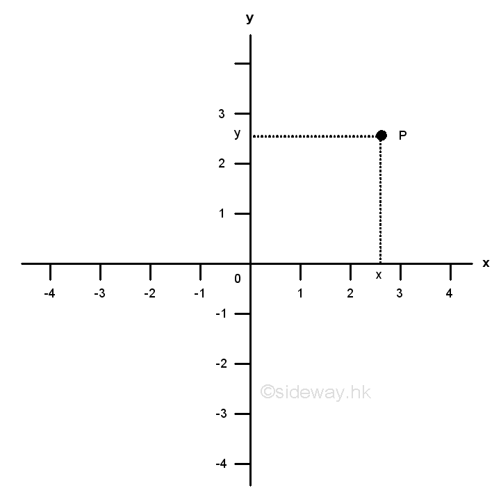
The graph of a function is a visual representation of the function by plotting all ordered pairs (x, f(x)) within the domain of the independent variable x on a coordinate system. One of the most common coordinate system used in a function graph plotting is the cartesian coordinate system. The Cartesian coordinate system is also called rectangular system. For a two dimension coordinate system, there are the two axes, named x-axis and y-axis. The two axes, which should be linear and mutually perpendicular, are the axes of two rectangular coordinates accordingly. Each point, e.g. Point P on the coordinate system should have a horizontal coordinate x and a vertical coordinate y. Since each point can be represented by a pair of number, usually denoted by order pair (x,y), each order pair (x,y) can also locate a corresponding point on the coordinate system plane. Therefore each order pair of the function y=f(x) can be represented by a point on the xy- coordinate plane with the abscissa, or horizontal coordinate, x-axis, of the point is the value of the independent variable x and the ordinate, or vertical coordinate, y-axis, of the point is the functional value, value of the dependent variable y. For example; 
The graph is a plot of y vs x for the function y=f(x) . The curve is created by joining the points of ordered pairs of the function y=f(x). The curve is a continuous curve because the function y is a continuous function on the whole domain. 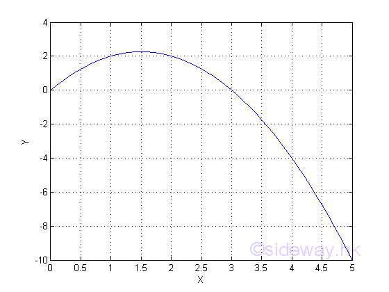
©sideway ID: 130100001 Last Updated: 1/13/2013 Revision: 0 Ref: References
Latest Updated Links
  Nu Html Checker Nu Html Checker  na na |
 Home 5 Business Management HBR 3 Information Recreation Hobbies 9 Culture Chinese 1097 English 339 Travel 45 Reference 79 Hardware 55 Computer Hardware 261 Software Application 213 Digitization 37 Latex 52 Manim 205 KB 1 Numeric 19 Programming Web 289 Unicode 504 HTML 66 CSS 65 SVG 46 ASP.NET 270 OS 431 DeskTop 7 Python 72 Knowledge Mathematics Formulas 8 Set 1 Logic 1 Algebra 84 Number Theory 206 Trigonometry 31 Geometry 34 Calculus 67 Engineering Tables 8 Mechanical Rigid Bodies Statics 92 Dynamics 37 Fluid 5 Control Acoustics 19 Natural Sciences Matter 1 Electric 27 Biology 1 |
Copyright © 2000-2026 Sideway . All rights reserved Disclaimers last modified on 06 September 2019